
I’ve been thinking about writing a blog post on what I have been doing these days. I thought, is there anything I can write about? Not just anything I learned, but something I can contribute to the public? And realized that few days ago I searched the web for a problem, but I couldn’t find the correct answer right away. Then I had to solve it myself. The problem is how to find margin lines from the decision boundary obtained from the linear SVM (Support Vector Machine) classifier.
This is not a hard problem to solve, but it needs a little bit of understanding on how SVM works. First, I will go through basic formula, and then get margin lines for two-feature cases.
If we have two continuous features, 


[


Let’s say we are using a python library, sklearn.svm.SVC. If we fit the training data, the package gives us optimal parameter values after solving above formula: coef_[0][0] as 
coef_[0][1] as 
intercept_[0] as 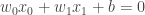


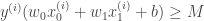
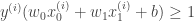
Then, 
Then a part of the python code for plotting these lines looks like this.
yy = -(w[0] / w[1]) * xx - (b / w[1])
yy_margin1 = yy + 1 / w[1]
yy_margin2 = yy - 1 / w[1]
I know this is not a hard problem, but it can be handy when we want to plot margin lines. (I found that some example codes at sklearn.svm.SVC were not correct at this moment, when they draw margin lines. One only works for separable cases, while the other one uses 
PS: All blog posts I have written so far (actually I haven’t written any for more than five years) are in Korean. So this will be my first blog post in English.
